Digital Twins: Quantifying Petrography (Pores, Grains)

1. Quantify OM Pores in the Marcellus Shale, Dry Gas, Lycoming County, PA (ML work completed by Ken Ikeda [2020]; Images and training datasets provided by Lucy Ko)

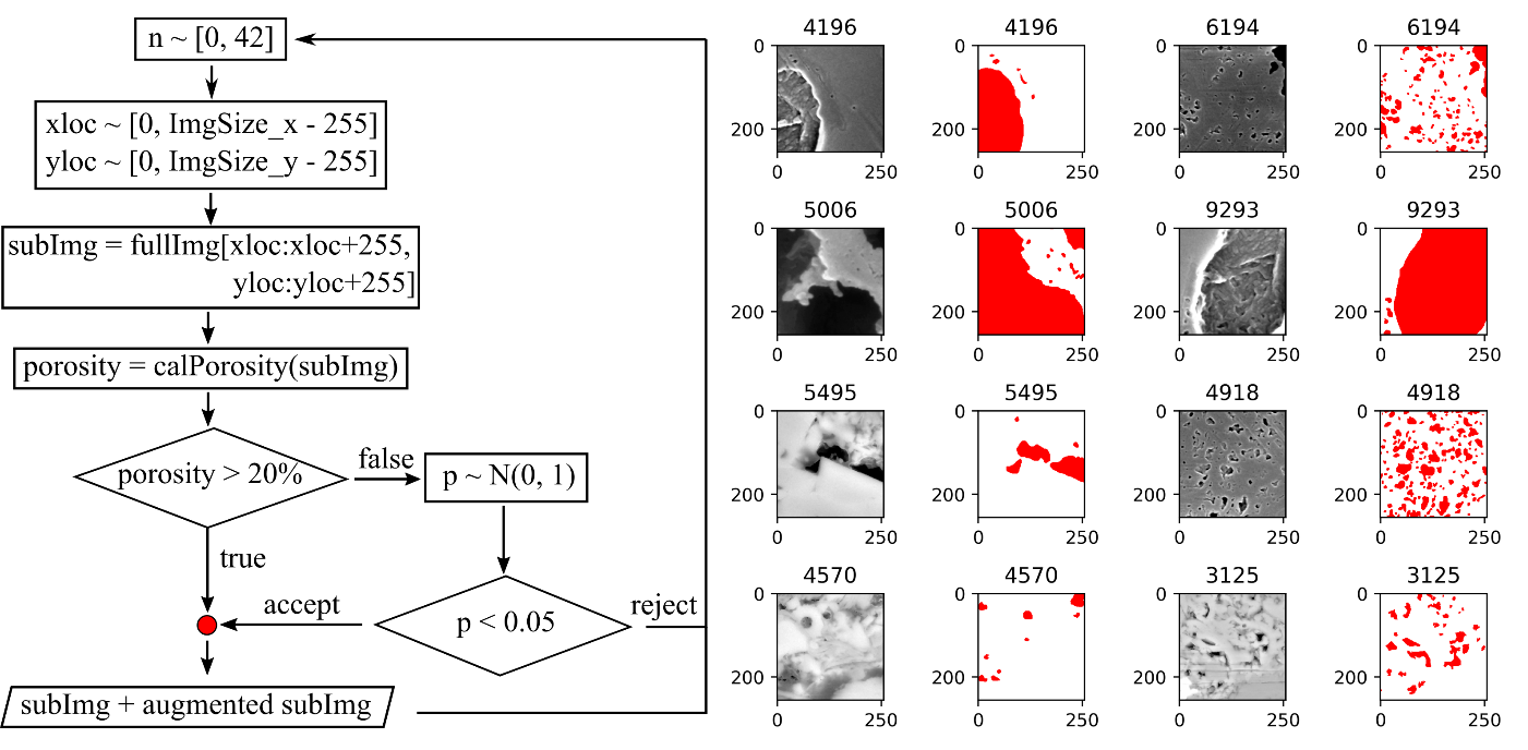
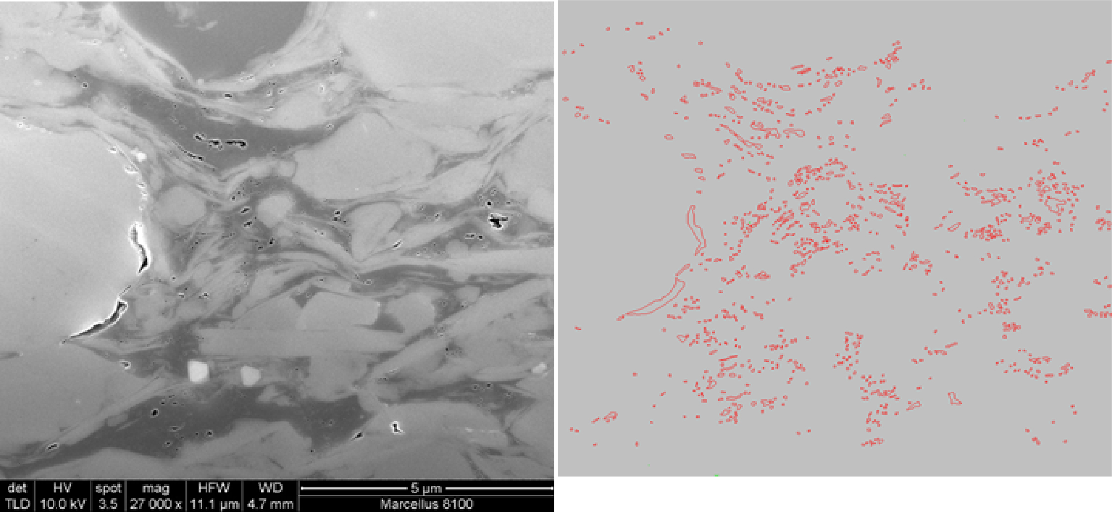
Fig 1.1 (left) A flowchart explaining the algorithm for extracting sub-images. (right) Examples of sub-images from the algorithm. — Figure 1.1 (left) A flowchart explaining the algorithm for extracting sub-images. (right) Examples of sub-images from the algorithm. Each of which contains a pair of an SEM image and its label. The number on top of each figure represents the number of the sub-image. The sub-image number 4570 is an example of a low-porosity sub-image, which was conditionally accepted from the criteria in step 5.

Fig 1.2 Marcellus Shale, training datasets of OM pores in solid bitumen and pyrobitumen, 8100 ft — Figure 1.2 Marcellus Shale, training datasets of OM pores in solid bitumen and pyrobitumen, 8100 ft (tracing credit: Michael Wang)

Fig 1.3 Marcellus Shale, resulting OM pores in solid bitumen and pyrobitumen, 8100 ft — Figure 1.3 Marcellus Shale, resulting OM pores in solid bitumen and pyrobitumen, 8100 ft

Fig 1.4 Marcellus Shale, OM pores in solid bitumen and pyrobitumen, 8138.08 ft — Figure 1.4 Marcellus Shale, OM pores in solid bitumen and pyrobitumen, 8138.08 ft

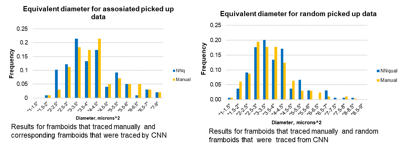
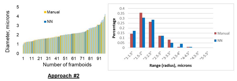
2. Quantify Pyrite Framboid Distributions in the Marcellus Shale, Dry Gas, Lycoming County, PA (ML work completed by Artur Davletshin [2020]; Images and training datasets provided by Lucy Ko & Priyanka Periwal)

Fig 2.1

Fig 2.2

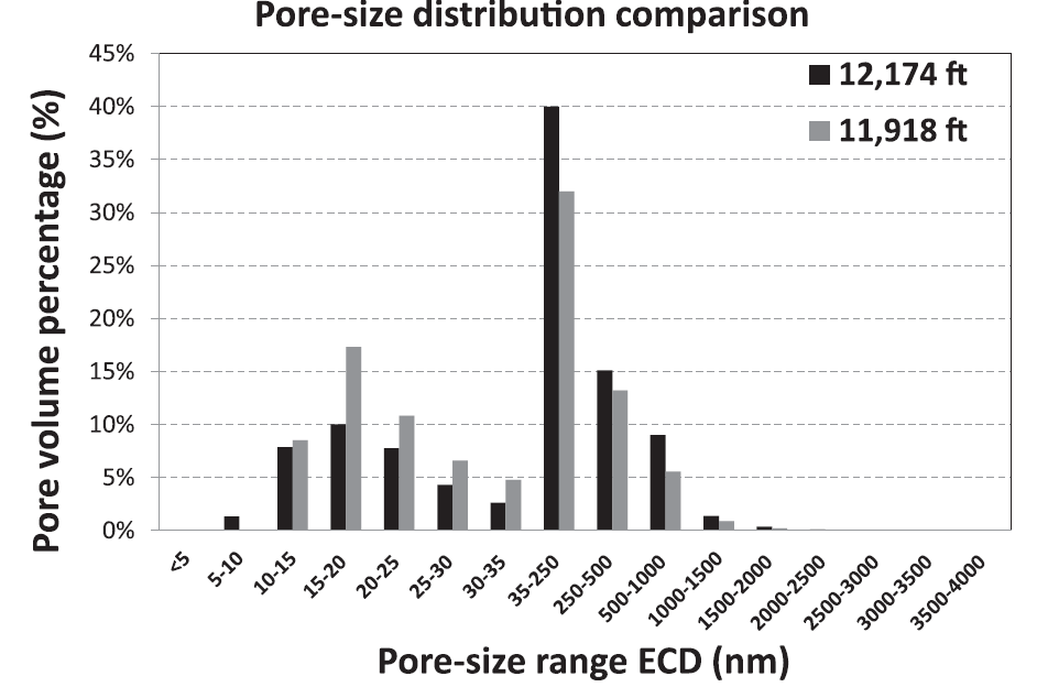
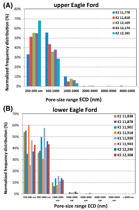
3. Quantify Pore-Size Distribution in the Cretaceous Eagle Ford Group, Karnes County, from SEM Images

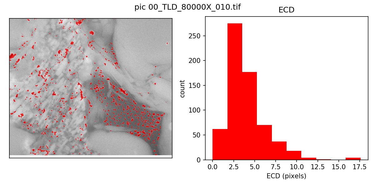
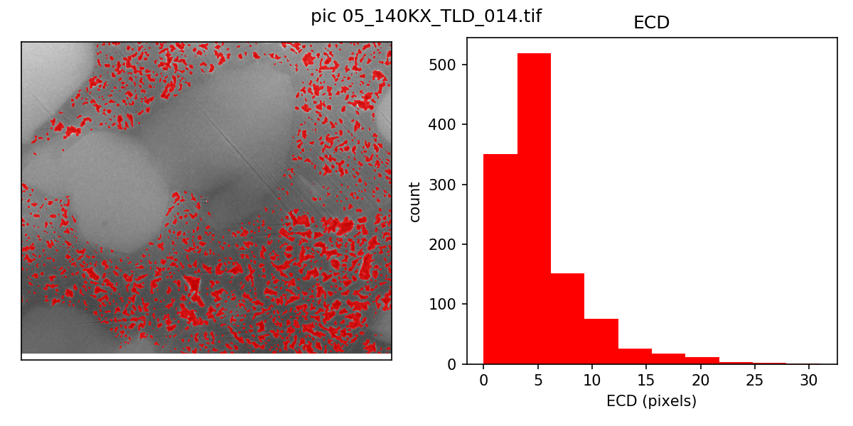
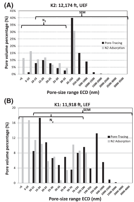
Fig 3.1 Plots showing comparisons of pore-size distribution in two marl samples — Figure 3.1 Plots showing comparisons of pore-size distribution in two marl samples (K1: 11,918 ft [3633 m], lower Eagle Ford; K2: 12,174 ft [3711 m], upper Eagle Ford) at 5000X, 15,000X, and 120,000X scales. ECD = equivalent circular diameter (Ko et al., 2017a)

Fig 3.2 Plots of normalized pore-size frequency distribution of marl facies — Figure 3.2 Plots of normalized pore-size frequency distribution of marl facies from (A) upper Eagle Ford (UEF) and (B) lower Eagle Ford (LEF) sections in K1 and K2 cores. Pore-size distribution data were obtained from manually traced pores on 5000 scanning electron microscope images. The frequency was normalized to 100% to compare differences. Note that, in the UEF, smaller pores are increasingly abundant with depth, whereas large pores show the opposite trend. No trends are apparent in the LEF. ECD = equivalent circular diameter. (Ko et al., 2017a)

Fig 3.3 Comparison of pore-size distribution of marl samples from pore-tracing and nitrogen-gas–adsorption measurement. — Figure 3.3 Comparison of pore-size distribution of marl samples from pore-tracing and nitrogen-gas–adsorption measurement. (A) Core K2: 12,174 ft (3711 m), upper Eagle Ford (UEF). The two techniques show very similar pore-size distribution. (B) Core K1: 11,918 ft (3633 m), lower Eagle Ford (LEF). Differences in the two techniques are largely resulting from the differences in scale resolution between the techniques. The two horizontal brackets indicate detectable ranges of each method.

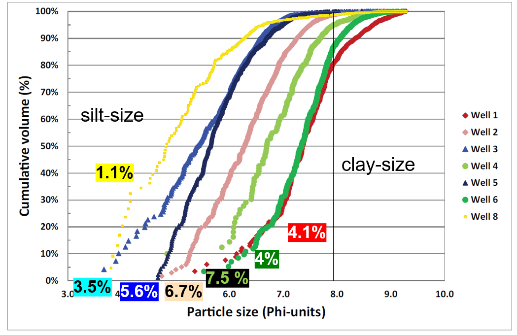
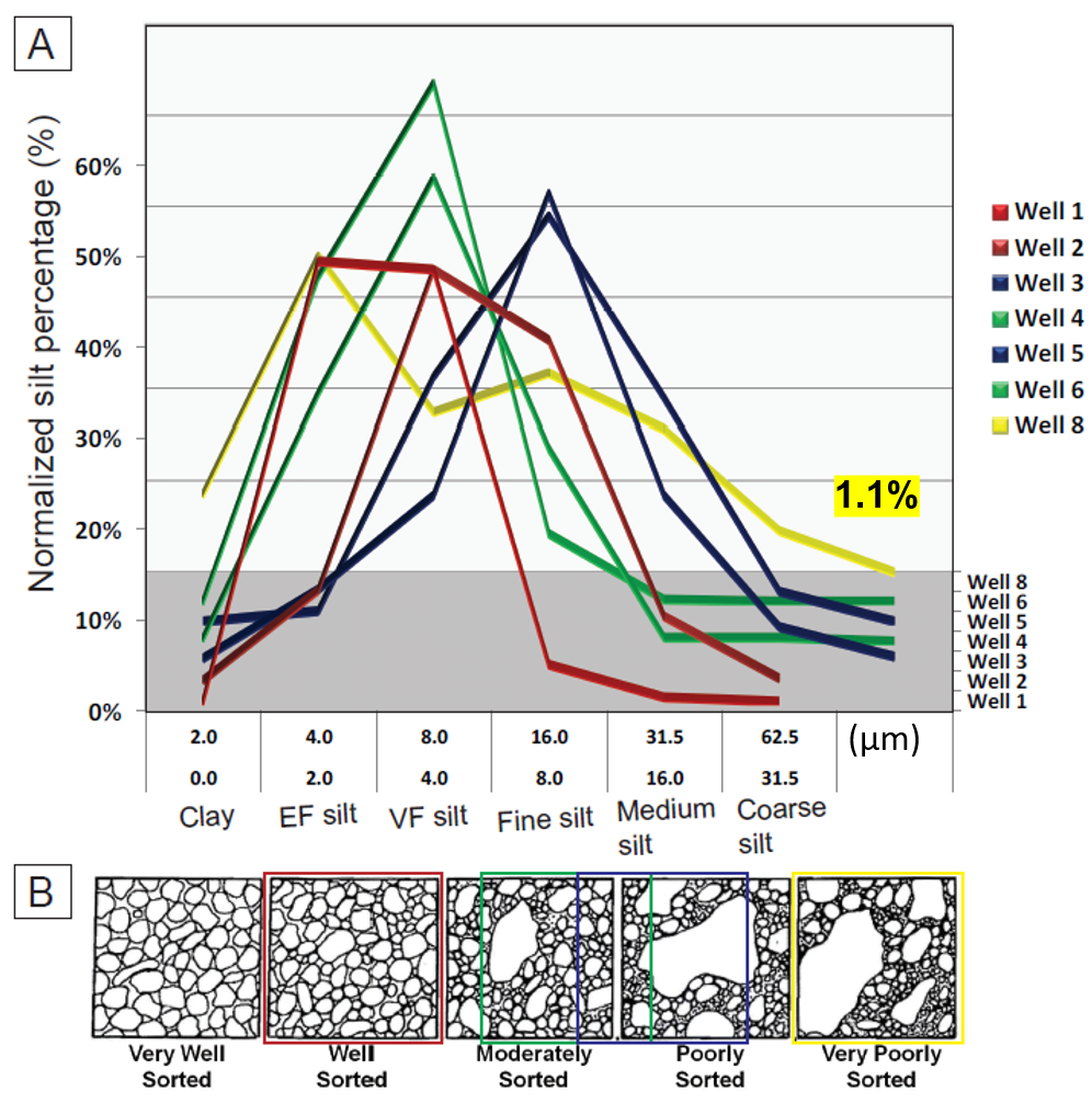
4. Quantify Grain size distribution and sorting in the Yanchang Formation, Ordos Basin, China (Lucy Ko [2017]): plots here demonstrate total clay mineral%, sorting, and grain sizes affect porosity and permeability

Fig 4.1

Fig 4.2 — (Ko et al., 2017)

© 2021 Bureau of Economic Geology | Web Privacy Policy | Web Accessibility Policy