Analyzing Initial Conditions for Fluid Contacts

The analysis of fluid contacts gives a starting point for analyzing reservoir production trends. To begin this analysis, the relative position of the data must be easily accessible. This is accomplished by the compilation of completion and workover information. Once these data have been compiled on maps, logs, and graphs, the initial analysis of fluid contacts begins.

Background
Initial fluid contacts in a reservoir are normally under static conditions. Under these conditions, the fluid contacts are determined by fluid density with gas over oil and oil over water. Contacts are also horizontal, which results in segregation of fluids by depth within a single body of rock (compartment) in which fluid is free to move. A significant number of reservoirs contain fluid-flow barriers that segregate the reservoir into compartments. Because the compartments are not in fluid-flow communication, each one can potentially have separate fluid contacts at different depths. Original fluid migration and structure control the location of fluid contacts within each compartment. Each compartment in a reservoir has a different possibility of being filled by hydrocarbons, depending on the amount of fluid migrating and how well it is connected to the source. Additionally, compartments may have different spill points, resulting in different fluid-contact depths. The reservoir is divided into separate compartments when multiple fluid contacts are present. Likewise the location of multiple fluid contacts can aid in the determination of compartments.

Methodology
Original fluid contacts are established in a reservoir by analyzing completion and test data, wireline logs, and pressure data. Completion and test data establish what type of fluid occurs at what depth. Wireline data are used to calculate the saturation of water and can also be used to detect the presence of hydrocarbons. Initial pressure data are analyzed to determine the hydrocarbon-water contacts in a normally pressured system.

Completion and test data are evaluated by posting fluid-flow test results at subsea depths on a structure map. The structure map should be drawn on the top of pay for each genetic unit. For each test that shows hydrocarbon flow, the lowest known oil (LKO) or lowest known gas (LKG) is calculated in subsea depth at the lowest perforation. These values are used to establish the depth of the hydrocarbon interval. For tests that show water flow, the highest known water (HKW) is established by calculating the subsea depth at the top of the perforation interval. With this information posted on a structure map, the range in which the fluid makes contact can begin to be delineated.

There are numerous ways to use wireline logs to evaluate the fluid type at any given depth. Resistivity logs can be used to establish water saturation, or combined neutron and density can be evaluated to detect the presence of free gas and contacts. Importantly, the wireline data should be calibrated with the production test information. Then the subsea depth of contacts and LKO, LKG, and HKW are determined from the wireline data posted on the structure map along with the test data.

When initial pressure data are analyzed, the hydrocarbon-water contacts in a normally pressured system can also be determined. The salient point to apply here is that at a fluid contact both fluids are at the same pressure. However, because different fluids have different densities, they produce different pressure gradients. Hydrocarbons are normally less dense than water, so they create smaller pressure gradients and steeper lines on a depth-vs.-pressure graph as a result (fig. 4 below).

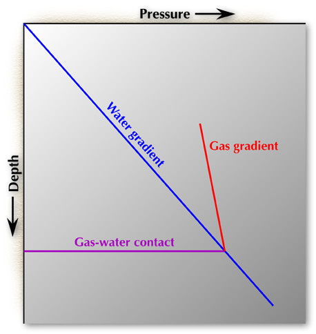
Figure 4. Water chemistry map displaying the variation of water resistivity and anion-cation concentration with the aid of stiff diagrams.

To determine the fluid contact in a normally pressured system, a line is drawn on the water-gradient line and on the pressure-vs.-depth line, and then the pressure measurements taken in the hydrocarbon fluid column are plotted. A straight line is then drawn through the points with a slope that would result from the density of the hydrocarbon. The intersection of the water-gradient line and the hydrocarbon line, where the pressure is equal, is thus the hydrocarbon-water contact.

If a hydrocarbon reservoir or compartment is suspected of being abnormally pressured, the fluid contacts cannot be determined by analyzing pressure. To determine whether a reservoir is normally or abnormally pressured, the fluid contacts must be known. To evaluate the character of a pressure system, the following steps are performed:

1) Gather and organize pressure and depth data for all wells, including the hydrocarbon-water contact (HWC) for each reservoir.

2) Generate pressure-vs.-depth graphs for each reservoir.

3) Annotate the HWC on each graph.

4) Fit hydrocarbon pressure measurements with a gradient line and extrapolate to HWC. Note that a typical oil gradient is 0.35 psi/ft, and gas is 0.08 psi/ft.

5) Record the pressure at the HWC and compare pressure with the normal hydrostatic pressure by applying:

P hydrostatic (psig) = 0.45 * Depth (ft) + C, where C is zero for a normally pressured reservoir.

It should be noted that because gas-pressure gradients are small, the reservoir pressure for a gas prospect could be estimated by applying the hydrostatic pressure gradient at the spill-point depth, as long as the prospect is normally pressured and the gas column is not overly large.