Activities
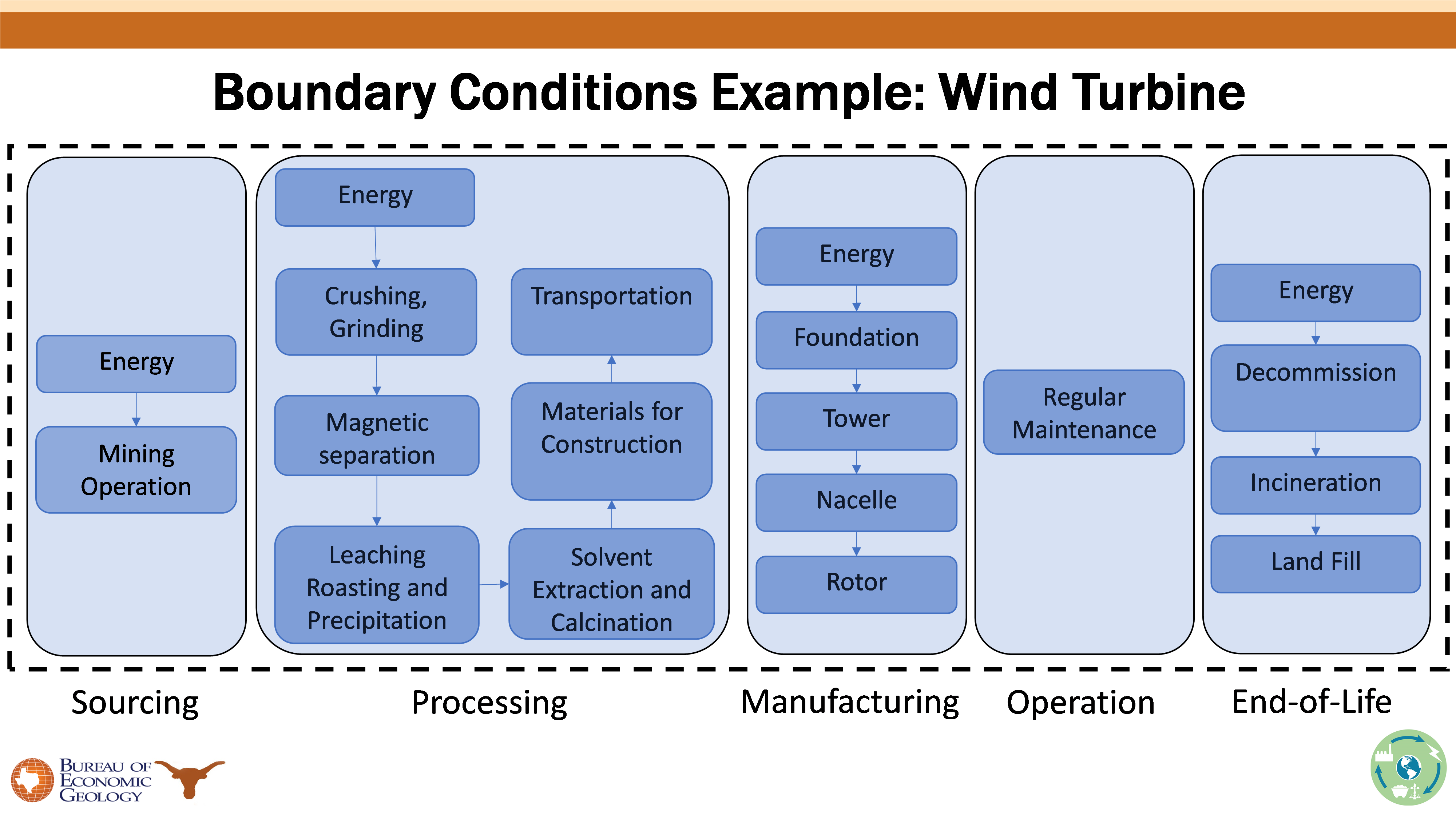
Cradle-to-grave boundary conditions: Our LCA boundaries includes all activities involved in extracting natural resources, processing them, manufacturing energy equipment, operations of the power plant and the disposal or recycling considerations at the end of useful life. The following is the example of this cradle-to-grave life-cycle for a wind turbine.
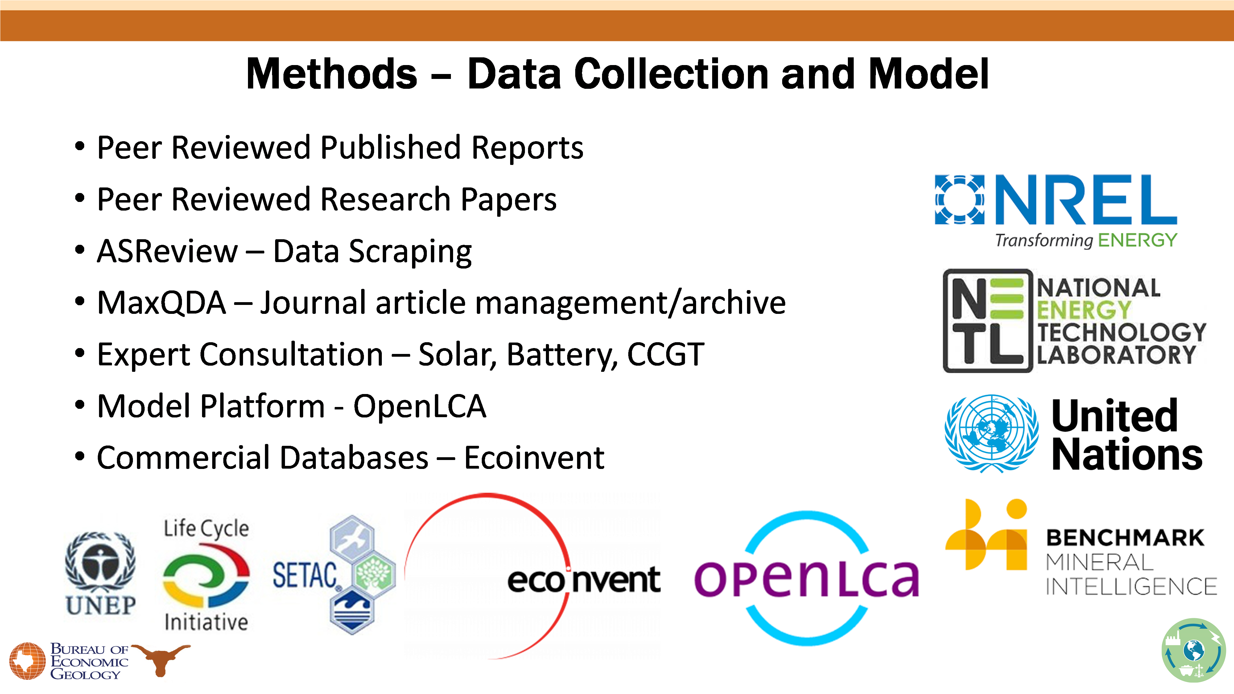
Data collection and analysis: we use existing databases on environmental impacts input parameters but we also supplement with data from most recent research and, where possible, from companies in the field.
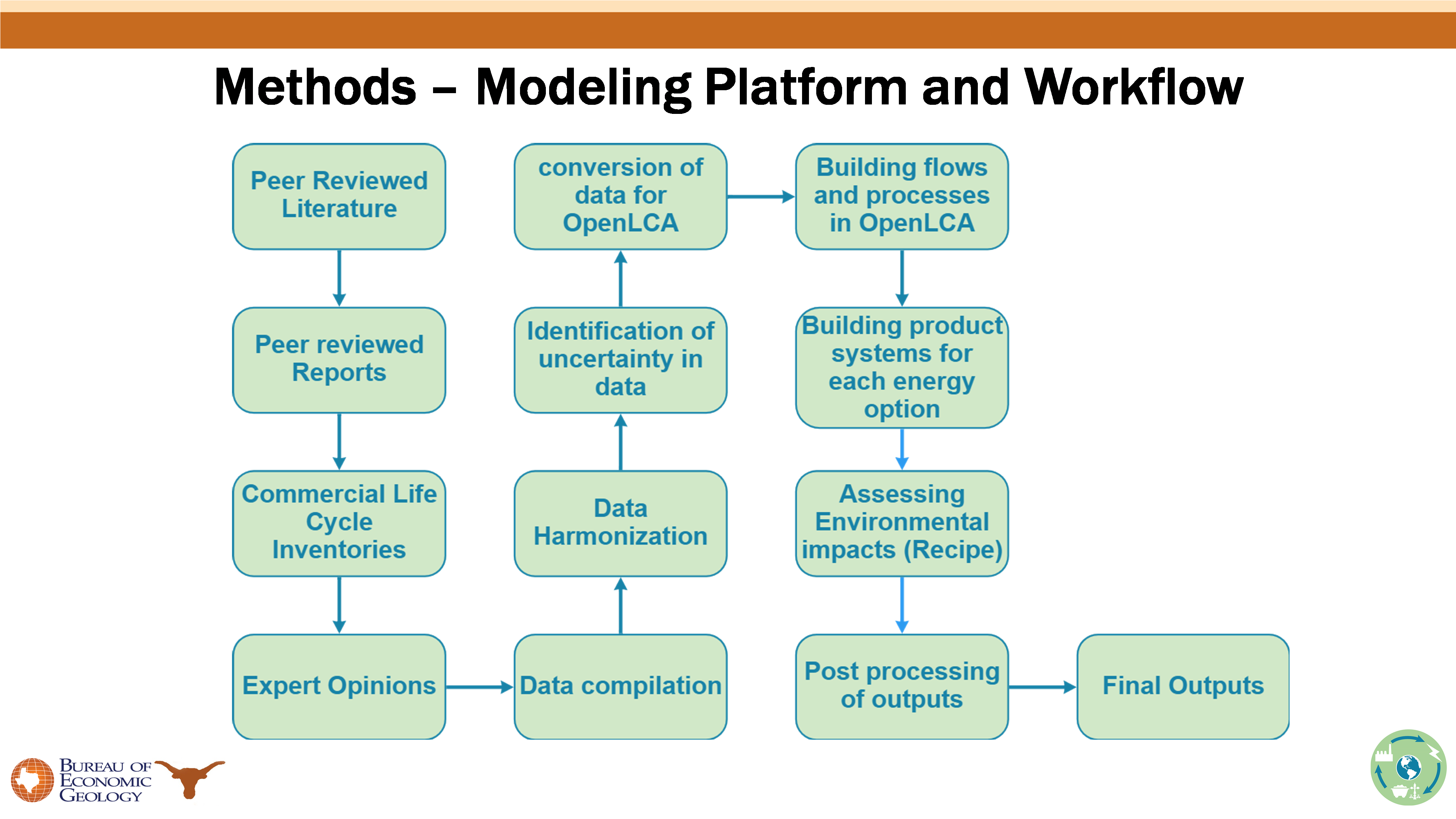
Workflow: A linear approximation of our workflow is depicted in the following graphic. In reality, we circle through different steps of this workflow multiple times to ensure recency of data and consistency of assumptions with actual industry operations.
Zachary Harner graduated with his master’s degree from UT Austin’s Energy and Earth Resources (EER) program. His thesis focused on the LCA across the lithium supply chain. In particular, he evaluated two scenarios on lithium supply chains as depicted in following graphics.
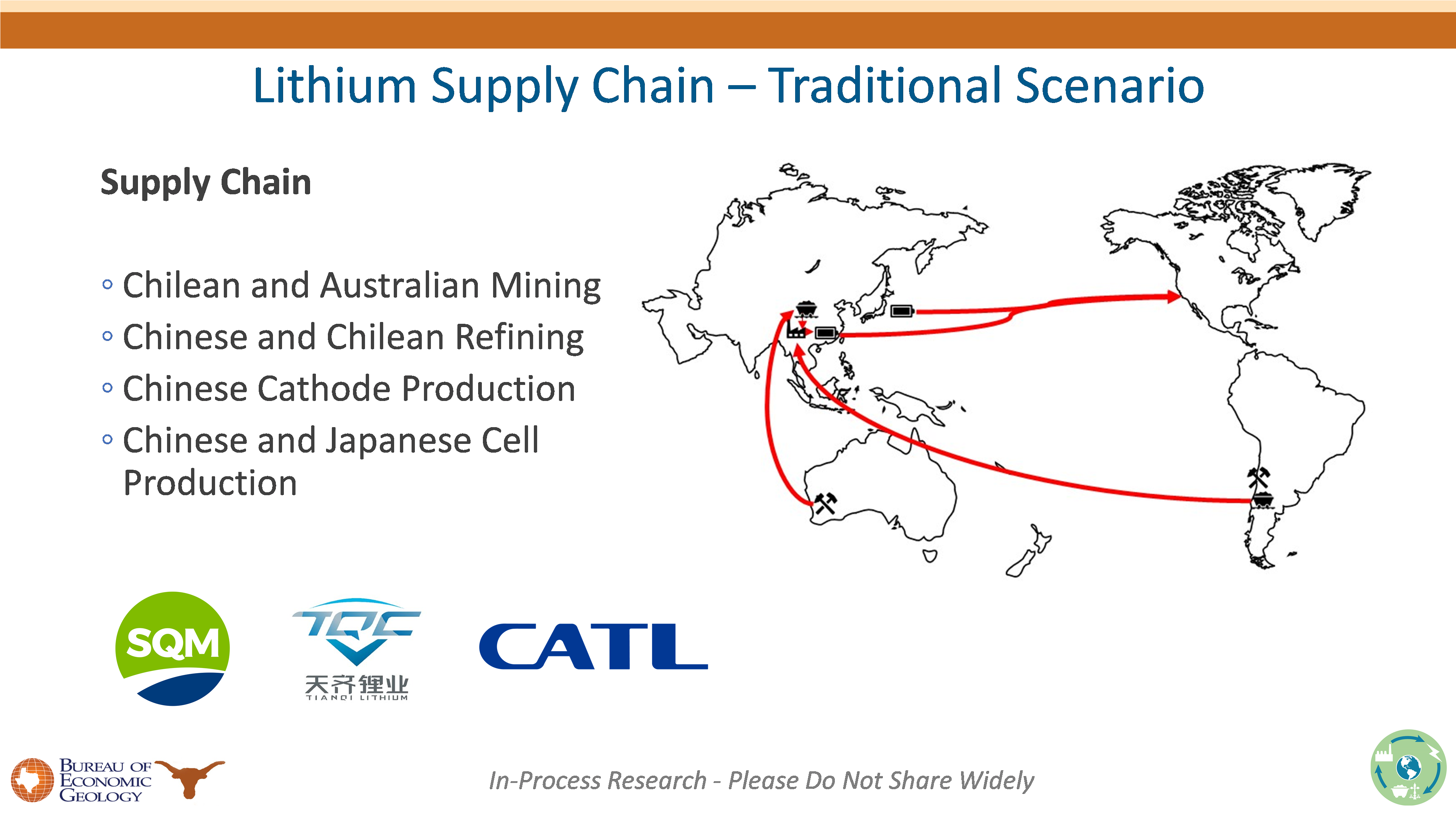
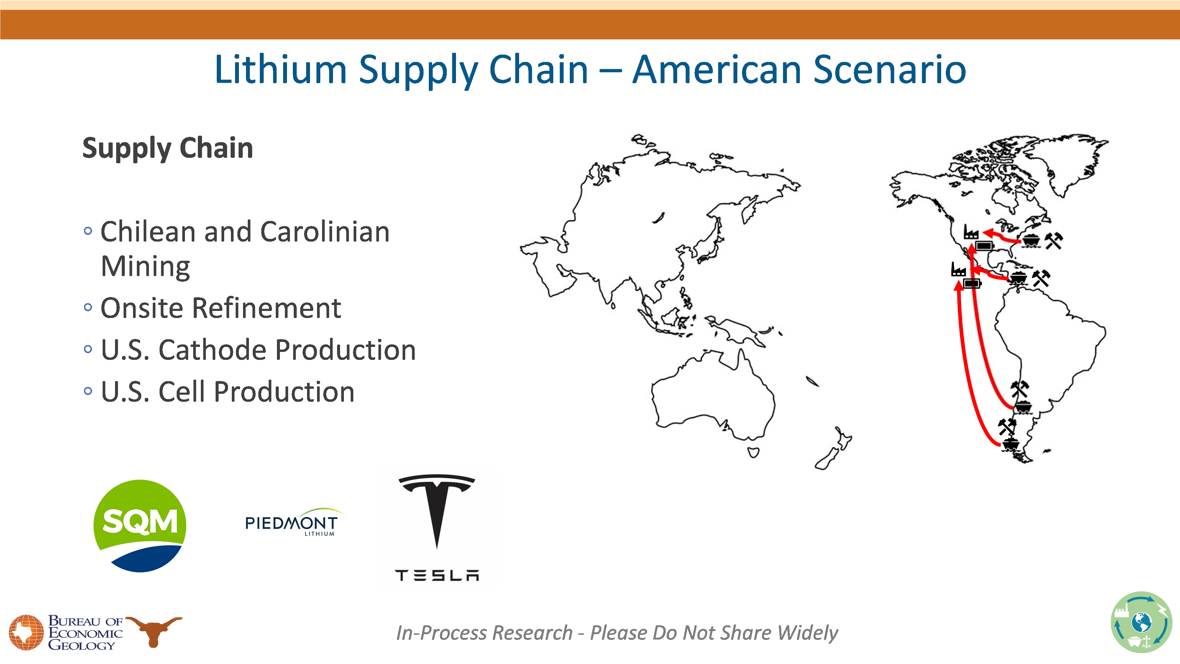
Zachary’s poster at the SME Conference provides further details on his research.
Andrew Kleiman graduated with his master’s degree from UT Austin’s Energy and Earth Resources (EER) program. His thesis focused on the LCA across the cobalt supply chain. In particular, he evaluated three major cobalt supply chains as depicted in following graphic.
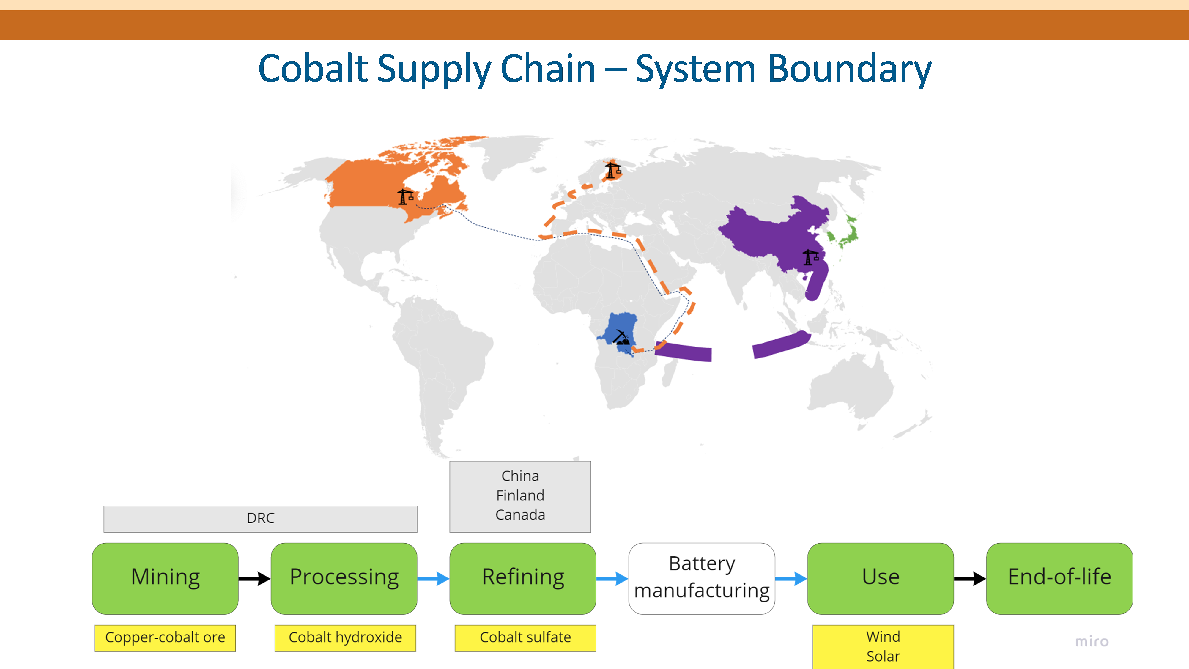
Andrew’s poster at the SME Conference provides further details on his research.
Hazal Kirimli, another EER student, shared early results in her poster on nickel supply chains at the SME conference.
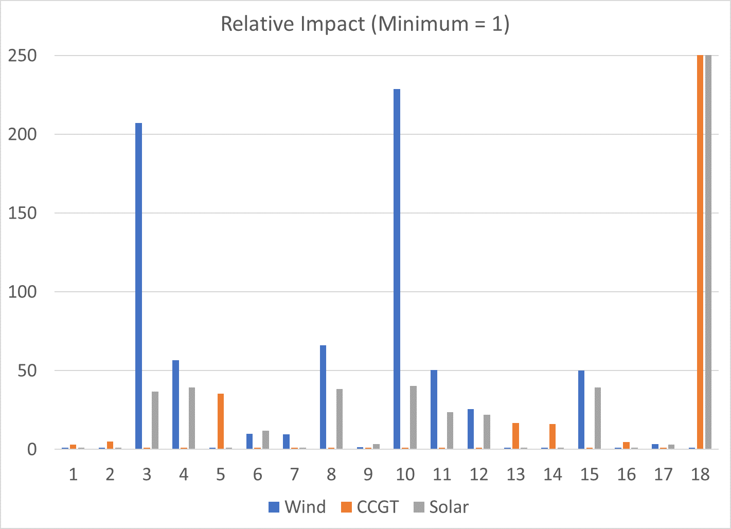
These figures demonstrate the importance of incorporating cradle-to-grave boundaries and all environmental impacts to identify areas in the supply change where impacts can be mitigated. For example, the following graphs compare where different impacts concentrate along the supply chains for two different generation technologies, capable of generating the same amount of electricity per year. The results are preliminary and provided for illustrative purposes only.
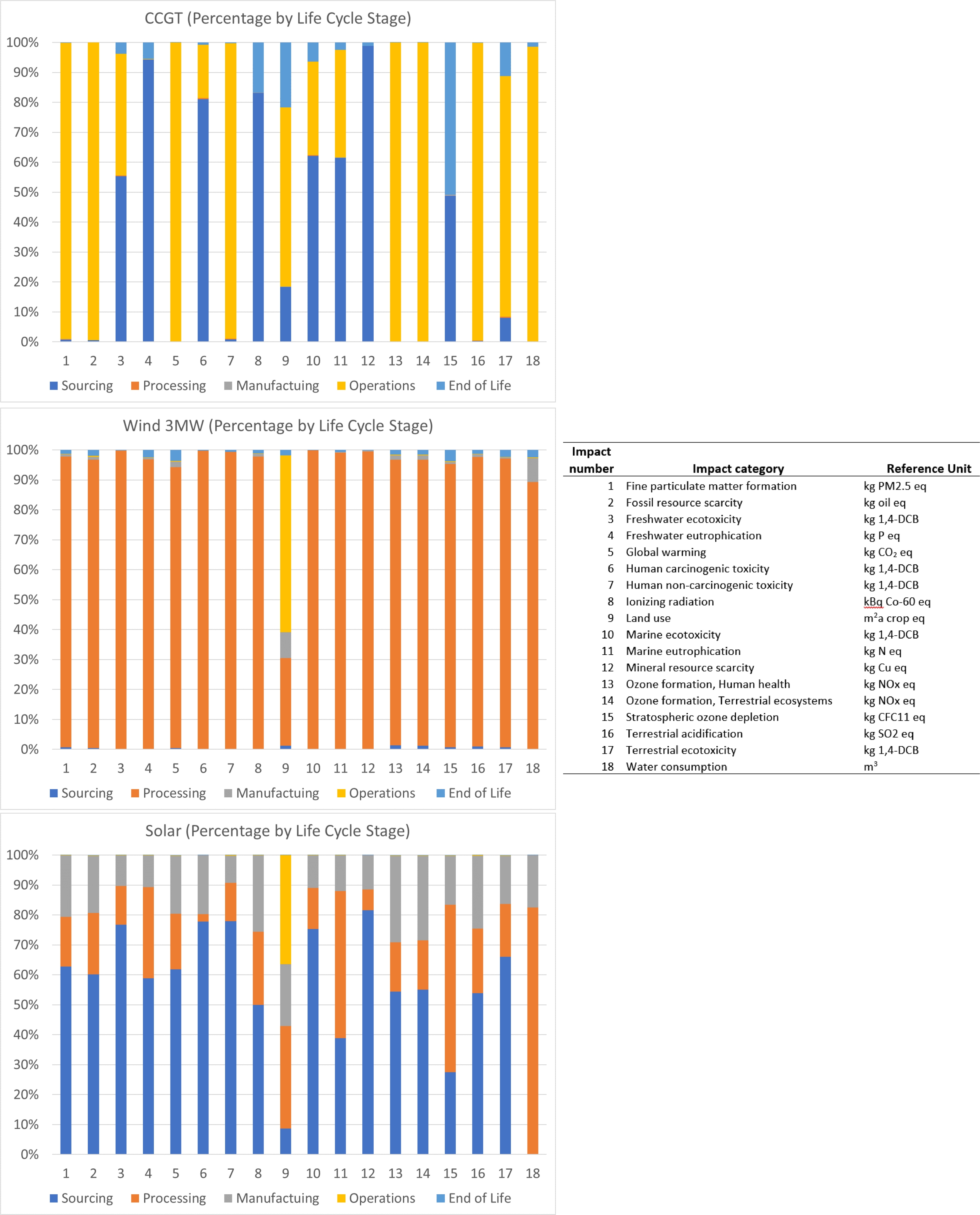
Note that:
- Supply chains are global, yet the impacts can be locally concentrated, dispersed across wider regions or global in scale. For example, impacts during operations are felt by communities near the power plant, whereas impacts during sourcing and processing of natural resources are felt by communities near extraction sites and processing facilities.
- Impacts have different units. Harmonizing all impacts into a one metric is difficult. For example, we represent all impacts relative to the minimum across the three generation technologies (see chart below). We continue to debate on alternative ways to report aggregate impacts in a meaningful way (e.g., economic costs of impacts).
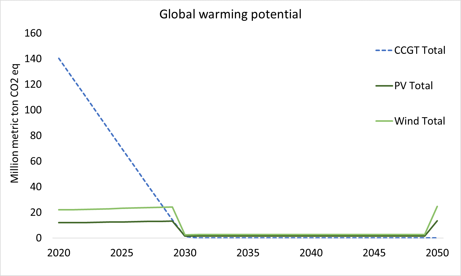
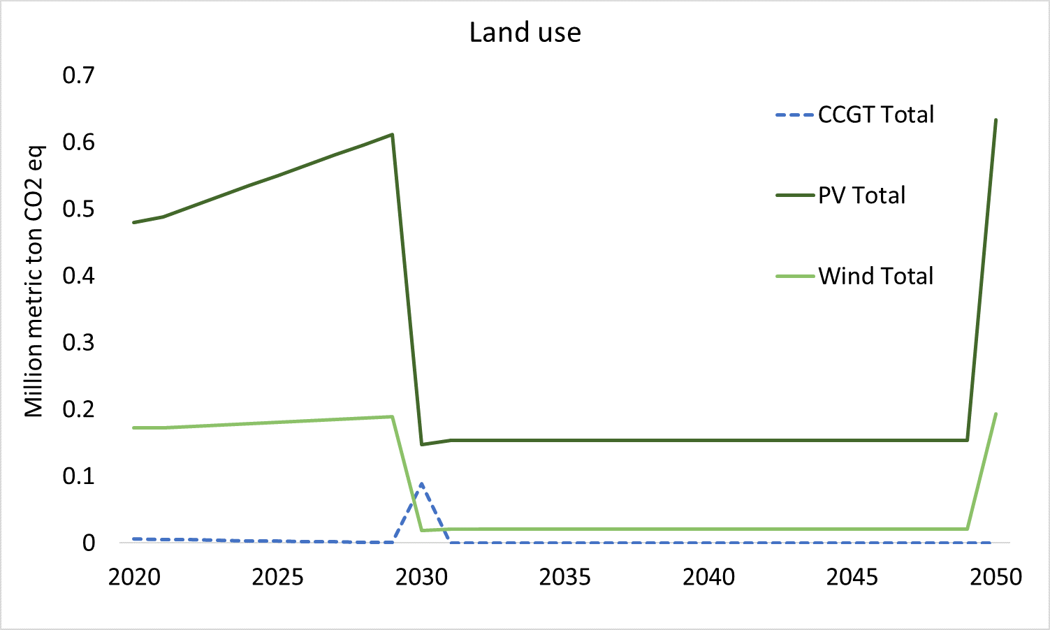
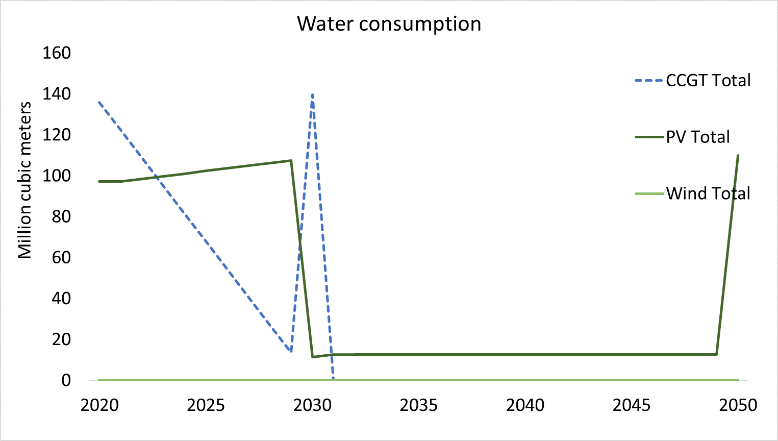
Temporal distribution of impacts is important for visualizing what to expect during transitions of electricity generation technologies. For example, the following graphs compare timelines of total Global Warming Potential (GWP), Land Use and Water Consumption across all phases in our system boundaries (i.e., including sourcing, processing, manufacturing, building and operating and EoL) that are associated with transitioning from a CCGT plant over 10 years to Solar PV or Wind technologies, each assumed to operate for 30 years.. Assuming shorter operational lives for solar and wind could cause periodic spikes in impacts. Changes in generation performance could also influence these timelines. The results are preliminary and provided for demonstration purposes only. We are working on developing similar representations for all 18 impacts considered in the LCA portion of our study.
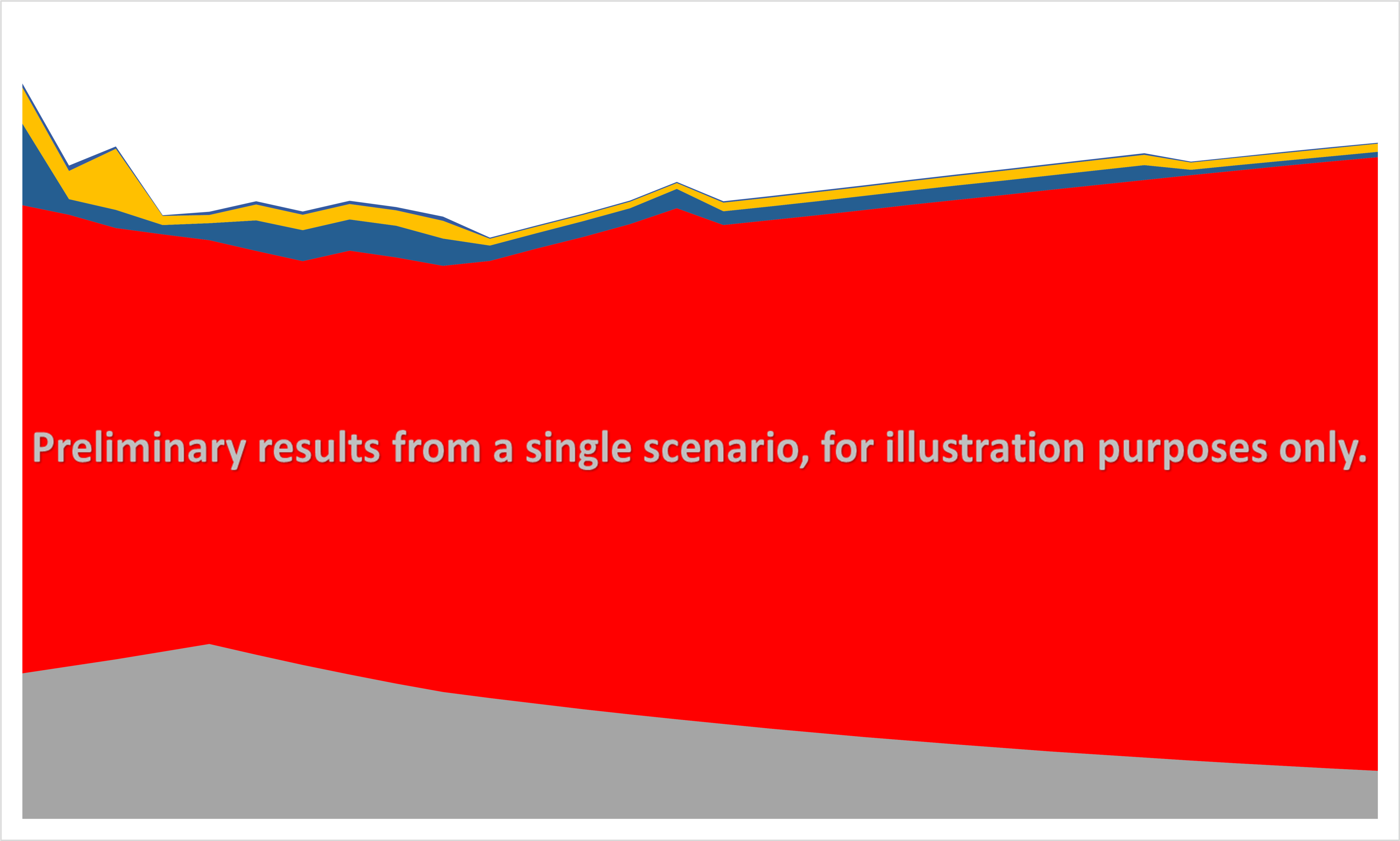
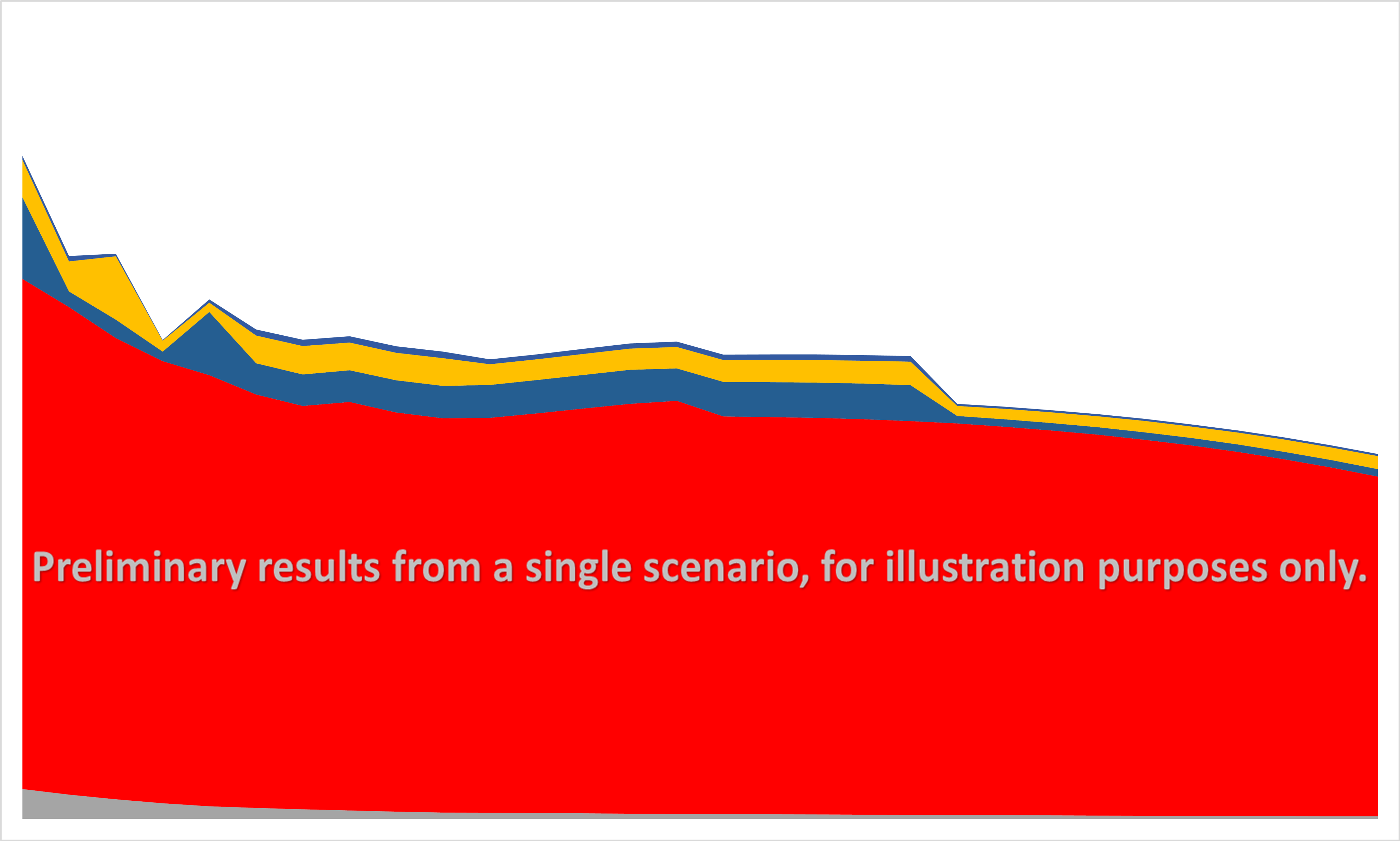
All of our power plants generate the same amount of electricity in a year. With battery storage, we bring solar and wind facilities closer to dispatchability to match a CCGT plant. Hence, our LCAs approximate total amount of materials needed for “equivalent” facilities. Still, this approach does not capture the needs of an electric power system that is expected to balance demand and supply of electricity in real time, instantaneously. In phase 2 of the CEO study, we aggregate LCA impacts calculated for individual power plants for whole power systems. That is, we include all generation and transmission and distribution (T&D) assets that need to be built and operated by 2050 under various scenarios. For example, the following charts compare the GWP impacts across two transitioning scenarios of energy generation portfolios in an actual power grid. We will confirm reliability of these systems via high-frequency (e.g., hourly) dispatch modeling.
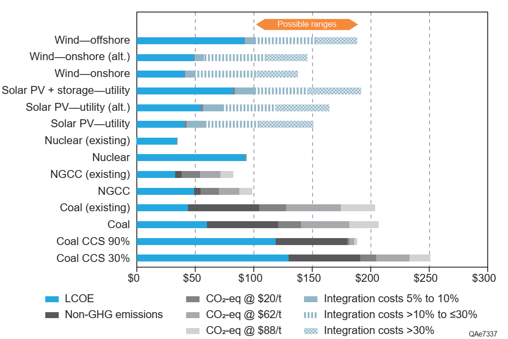
In phase 3 of the project, we will offer an alternative to LCOE as a more comprehensive representation of the total social cost of electricity to consumers. In addition to conventional capital, operating, fuel and financing costs, we will include system integration costs associated with new T&D and reliability infrastructure, and economic costs of externalities (i.e., all 18 categories of the LCA). The following is an example from previous work. See Net Social Cost of Electricity or USAEE podcast. We are working on alternative approaches to a more inclusive metric of electricity costs with other interested parties.